Adding Noise The Analytic Graph
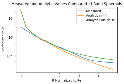
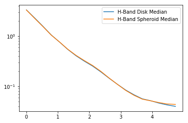
H Band Spheroid Median plotted with Disk Median
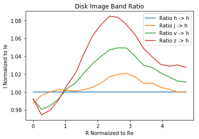
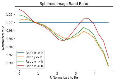
Ratio of Bands
Fitting with a Gaussian Process
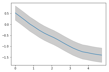
We’ll fit using the data from the Disk class in the H-Band which looks like this after we moved the data to log scale:
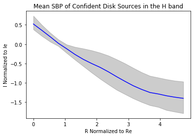
The data is heteroskedastic, we’ll remedy that by taking the mean of the difference between the $84^{th}$ percentile and the median.
To fit the Gaussian process we’ll use the following kernel function:
Where $\sigma_f$ is a parameter that controls the variance and $l$ is the length scale parameter.
With the paramters, we can predict new values using the following:
Where $K=k(x,x)+\sigma_n^2\delta(x,x’)$, $K_*=k(x,x’)$, and $K_{**}=k(x’,x’)$
The best predicted value for point $y_*$ is the mean of the distribution:
And the uncertainty is in the variance of the distribution:
With the fitted paramters and the calculations to make predictions, we can now sample from this process to create images.
To sample unique value we introduce some noise to $\textbf{y}$ by adding from a normal distribution with $\sigma=\sigma_n$. Although this may cause the observed values to be more jumpy, they should still be within an acceptable range, and the sample we draw from will tend to be smooth as a result of the Gaussian Process.
Using the new data we will use the Gaussian Process to predict $I_e$ normalized intensities at different $R_e$ normalized radii.
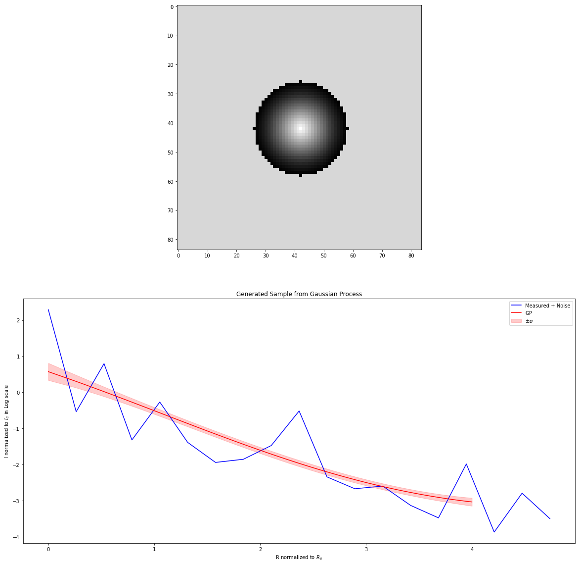
To generate an sample image we choose the paramters, $I_0$, $R_e$, $R$, then we draw a sample from the Gaussian Process getting $y_*$ for each pixel’s radus value normalized to $R_e$
For example if we set: $I_0=1$, $R_e=0.24$ $R=4.0$, the scale arcsecond/pixel = $0.06$.
We get this source and surface birghtness profile in log scale.: