Goal
Fit a Gaussian Process to the data set of images we have to create images that synthetic images that are from the same distribution.
Process
- Get all sources where we are confident about the label spheroid/disk. Confident means ($\Pr(class=argmax_1) - \Pr(class=argmax_2)\geq.5$)
- Get data in terms of $I_e$ and $R_e$
- Fit Gaussian Process to distribution
- Create synthetic images using a realization of the fitted Gaussian Process
Get data in terms of $I_e$ and $R_e$
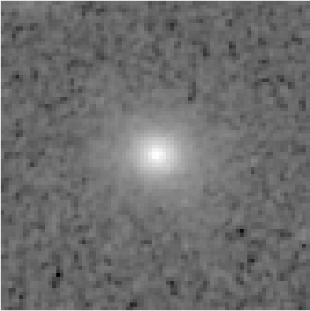
Start with the image(deep2_10521, h band, viewed in log scale) and its segmap.

Get $I_{tot}$ by measuring the flux in the area of image where the segmap defines the source
Find the maximum point in the segmap area and use that as the center of the source.
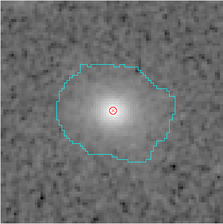
Starting from the center of the source measure the flux until it reaches at least $\frac{I_{tot}}{2}$ . Then, record that radius as $R_e$ and the mean values of the pixels in that radius as $I_e$.
Then normalize the data to $R_e$ by dividing all radius values by $R_e$ and normalize the data to $I_e$ by normalizing all $I$ values by dividing them by $I_e$
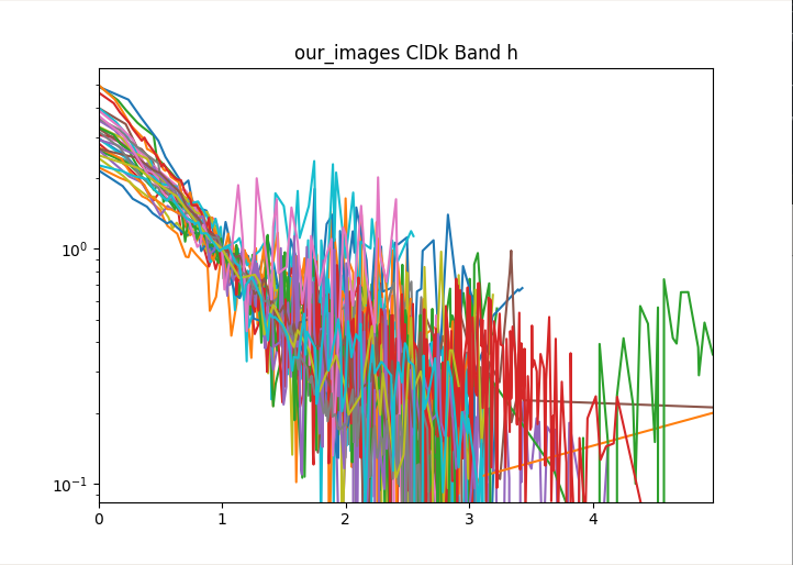
After recording this for all of the confident spheroids and disks, we then radially bin the normalized $I$ values by the normalized $R$ values.
Here’s the graph for 30 objects from the dataset. The graph gets pretty messy with larger numbers.
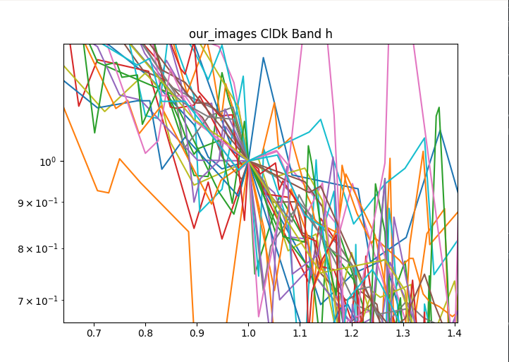
The data is normalized to $I_e$ and $R_e$ so if we zoom in to the value 1 for $I_e$ and $R_e$ we see that all of the data lines pass through that point.
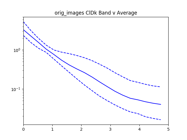
With all the values we then plot the $84^{th}$, $50^{th}$.and $16^{th}$ percentiles from the objects rank ordered by brightness.

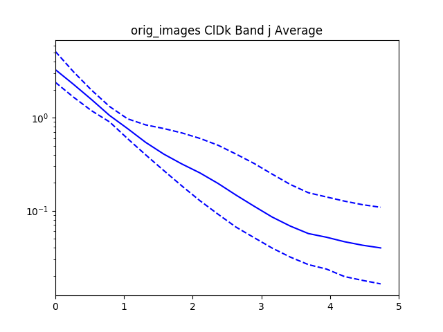


For reference added in is an analytic disk and spheroid created without noise. For the disks we used the mean measured $R_e$ and $I_e$ from the data. For the spheroids we had to hand pick $R_e=1.2$ and $I_e=0.01$, using the mean measured values caused the algorithm to measure an $R_e=0$ because of the steep gradient in the De Vaucouleurs sersic profile.
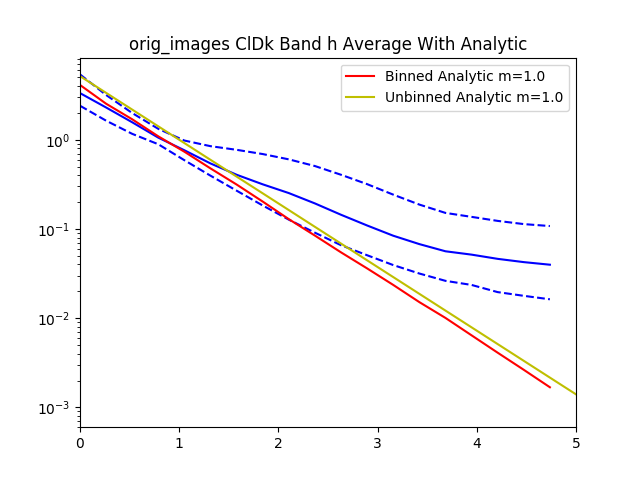
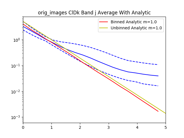
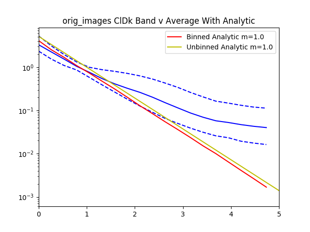

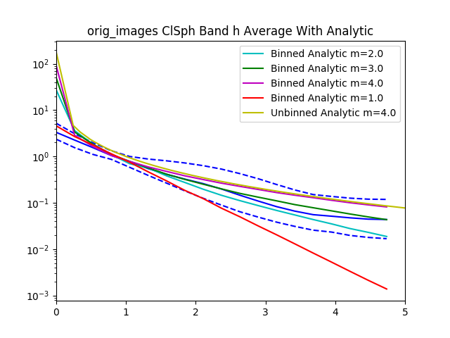

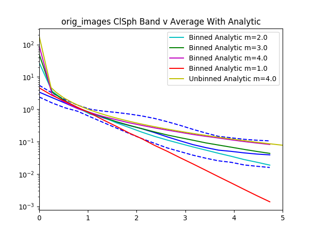
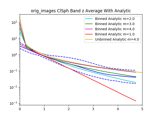
Interestingly, the spheroid data seems to more closely follow an exponential profile, however it could be that the noise in the image smooths out the data.
Fit Gaussian Process to Distribution
//TODO
Create Synthetic Images from Gaussian Process
//TODO